How to use pyPEAKO
Expected spectra file format
Creating training data
Training data contains the locations of peaks in cloud radar Doppler spectra, which have been marked by a human user. To create training data, spectra files must be in the cloudnet specific netcdf format. A sample is provided in sample_spectra.nc. Let’s use the sample data set to create some training data.
import pkg_resources
data = pkg_resources.resource_filename('peako', 'sample_spectra.nc')
data is a string which contains the path to the sample data file. Now we can load it into a TrainingData object:
import peako
P = peako.TrainingData([data], num_spec=[10])
We pass the location of sample data to the TrainingData object in a list (which can contain the paths to several spectra files). For this purpose, we only want to mark peaks in 10 spectra by hand. If we don’t set num_spec, this number is left at the default value, which would be 30. We can also set the maximum number of peaks to be marked when initializing the TrainingData object. The default is 5. Now we can mark peaks in Doppler spectra:
P.mark_random_spectra()
This will open a plot in a pop-up. Spectra are drawn randomly from the spectra netcdf file and plotted for marking peaks. If this doesn’t work, try playing around with the matplotlib settings, i.e. declare matplotlib.use(‘TkAgg’) in your script before calling mark_random_spectra. The pop up will look something like this:
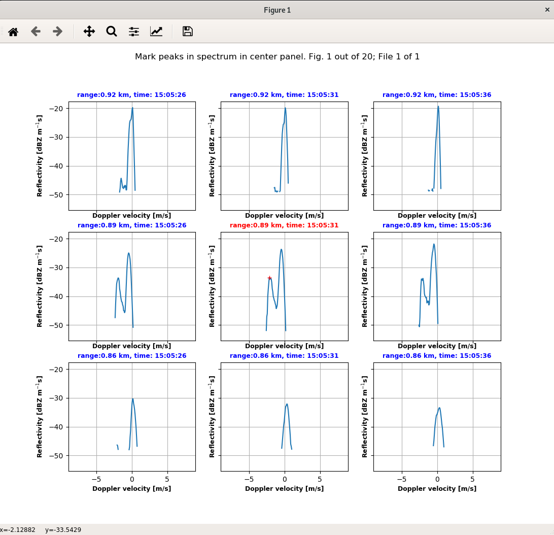
Screenshot of the GUI used for marking peaks by the user.
Mark the peak(s) in the plot in the center panel. Red markers will show you the points you marked. Use right-click to remove the previous mark if you want to change the location of the peak. Then hit Enter. If there is no peak in the spectrum displayed, hit Enter without marking peaks to move on to the next spectrum. You will get as many spectrum plots as you specified in num_spec in the previous step.
In the final step, we have to save the training data:
P.save_training_data()
This will create a netcdf file named marked_peaks_[name_of_specfile].nc in the same folder containing the spectra netcdf file. If such a netcdf file already exists, i.e. when you created training data already with the same spectra file, the found peaks will be added to the existing file.
Training the algorithm
PEAKO will use the user-marked peaks passed to the Peako() object for training. For detection of peaks, spectra are averaged both in time and height using a variable number of neighbors in time and range dimension. In the next step, smoothing of the averaged spectrum is performed. The method for smoothing is set in the Peako() object. ‘loess’ smoothing (locally estimated scatterplot smoothing), which is also referred to as Savitzky-Golay filter, is the default smoothing method (scipy.signal.savgol_filter(polyorder=2) ). In this averaged and smoothed spectrum, local maxima are detected, again using the scipy.signal toolbox. Maxima which don’t fulfill the requirements of minimum peak prominence or minimum peak width are discarded. During training, PEAKO looks for the combination of number of “neighboring” spectra in temporal and spatial domain over which to average, the span used for smoothing, the minimum peak prominence and minimum peak width, which best reproduces the user-marked peaks. The similarity between user-marked and algorithm-detected peaks is a measure based on the overlapping area below the spectrum. Different options for training are available:
- looping over all possible parameter combinations of time averages, range averages, span, width and prominence
- differential evolution from the scipy.optimize toolbox
Again using the example data provided in the package, we can set the Peako() parameters:
training_data = pkg_resources.resource_filename('peako', 'marked_peaks_sample_spectra.nc')
Q = peako.Peako([training_data])
Q.optimization_method = 'loop' # 'scipy' to use differential evolution from scipy
Q.training_params = {'t_avg': range(2), 'h_avg': range(1), 'span': np.arange(0.005, 0.02, 0.005),
   'width': np.arange(0, 1.5, 0.5), 'prom': range(2)}
The training_params set in the dictionary are defined as follows:
- t_avg and h_avg: number of neighbors each side over which temporal/ spatial averaging is performed. I.e. if h_avg is set to 1, averaging over three range bins will be performed with the spectrum of interest in the center range bin.
- span: the span which is used for loess or lowess smoothing from the scipy.signal toolkit
- width: minimum peak width in m/s
- prom: minimum peak prominence in dBZ
If optimization_method is set to ‘scipy’, the minimum and maximum of each of the dictionary items are used as bounds for the search. In the next step, we can train the algorithm:
result = Q.train_peako()
This will return a dictionary with the parameter combination of t_avg, h_avg, span, width and prom which yielded the best agreement with the training data. The parameter combinations which have been looped through, together with the respective similarity, are stored in Q.training_result.
We can also train Peako another time on the same data using differential evolution to see the difference it makes:
Q.optimization_method = 'scipy'
result_2 = Q.train_peako()
Caution, this may take a while.
Evaluating the training result
pyPEAKO has an in-built function for evaluating the training result, which can be called via
Q.training_stats(make_3d_plots=True)
By setting make_3d_plots to True, pyPEAKO will generate some 3D plots to show the effect of the different parameters on the resulting similarity.
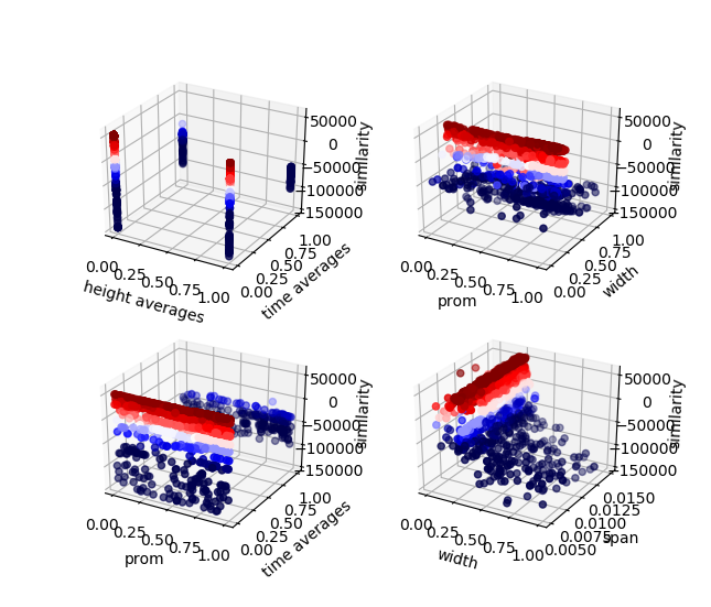
Example 3D plots of two variables (x and y axes) versus similarity (z axis)
We can also look at a couple of example spectra, in which the user has marked peaks by hand, along with the algorithm-detected peaks.